(LP secondary model) Modeling post cut-off cash flow to secondaries model

Secondaries Academy (LP Secondary Model) Modeling Post Cut-Off Cash Flow to Secondaries Model

Basic Concepts If you want the Excel backup file, please leave your email in the comments section.

While the secondaries market has experienced impressive growth over the last 10 years, little is known about actual secondaries modeling. That’s primarily due to the lack of publicly available knowledge.

In this post, we will explain how to model post-reference date cash flow into a secondaries model and what the implications are.

To level set, here are some basic concepts:

• Reference date: The GP’s valuation date. GPs typically value the portfolio on a quarterly basis.

• Closing date: When all legal documents are finalized. Both parties need to complete transfer documents, and funding must be wired by this date.

In most LP secondary deals, the base price is based on the reference date NAV (net asset value), and secondary buyers apply a discount to it.

The private equity market is illiquid in nature and requires significant time for buyers and sellers to agree on asset transfers. They not only have to agree on pricing but also complete operational due diligence and obtain approval from GPs. Usually, it takes weeks to months for both sides to agree on terms and close the transaction.

Between the reference date and the closing date, a lot can happen. The GP might sell companies in the underlying funds or make new investments.

In these cases, the question arises: who owns the cash flow from the underlying fund? Do distributions go to sellers or buyers? Is the seller or buyer responsible for funding new investments?

The industry-standard practice is that buyers are responsible for both post-reference date distributions and investments. You can think of it as if distributions are directly sent to the buyer, and buyers use that cash flow to reduce their bid price.

Scenario

• You are trying to purchase a $100mn commitment out of a $10bn fund, representing 1% of the fund’s total commitment.

• The fund has called $80mn out of the $100mn commitment, meaning it is 80% funded as of the reference date.

• You are willing to pay 90 cents on the dollar for the fund interest.

• There were $20mn in post-reference distributions.

• The asset grew by 10% between the reference date and the closing date.

With the $20mn distribution, your purchase price is reduced by $20mn ($100mn * 90% - $20mn). Therefore, your net purchase price is $70mn.

Your adjusted NAV—what the portfolio is actually worth—is also reduced by $20mn. Since the asset has grown by 10%, adjusted NAV should be $90mn ($100mn NAV - $20mn distribution + $10mn).

Now, what’s the implication?

Your actual discount is greater than the bid discount.

• Discount (without distribution): You are buying a $110mn stake for $90mn → actual discount is 18%.

• Discount (with distribution): You are buying a $90mn stake for $70mn → actual discount is 22%. → That’s a 4% difference.

Your asset is marked above 1x from day one.

• Day 1 mark-up (without distribution): $110mn / $90mn = 1.22x

• Day 1 mark-up (with distribution): $90mn / $70mn = 1.29x

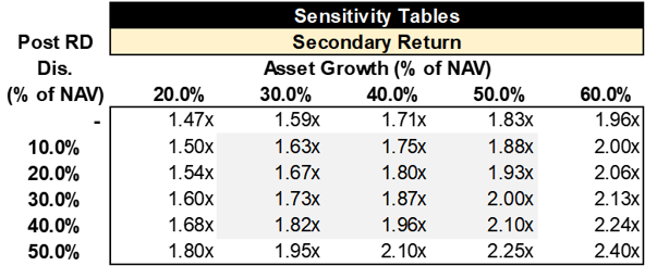
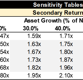
Your secondary return improves. Let’s assume the portfolio value increases by 40% at exit.

• Return (without distribution): $154mn ($110mn 1.4x) / $90mn = 1.71x Return (with distribution): $126mn ($90mn 1.4x) / $70mn = 1.80x

Does this matter when buying the portfolio? Under normal circumstances, it matters to a certain degree but less than the quality of the portfolio itself.

However, it becomes more meaningful when there’s a large post-record-date distribution. For example, using the same scenario, if there were a 50% NAV distribution post-record date, the difference would be significant. This is especially relevant for tail-end funds.

Why should you know this? It’s not a must, but knowing this will definitely impress your interviewers.